‌

Plotting

Mathematica has a host of different plot functions, but usually one only needs three of them:

Plot

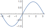
Plot takes a function as its first argument and a variable and range as its second one. Example:

Plot[Sin[x], {x, -π, π},
 ImageSize -> Small]

(*Out:*)

The function can also be defined outside of the Plot function itself:

sinx = Sin[x];
Plot[sinx, {x, -π, π},
 ImageSize -> Small]

(*Out:*)

User defined functions are also valid, but they must first be called on the variable one wants to use.

That’s why the following fails:

mySin[x_] := Sin[x];
Plot[mySin, {x, -π, π},
 ImageSize -> Small]

(*Out:*)

But the following will work:

mySin[x_] := Sin[x];
Plot[mySin[x], {x, -π, π},
 ImageSize -> Small]

(*Out:*)

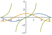
Plot can also plot many functions simultaneously, if the first argument is a list of appropriate functions:

Plot[{Sin[x], Cos[x], Tan[x]}, {x, -π, π},
 ImageSize -> Small]

(*Out:*)

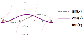
These functions can be distinguished from each other via legends and styling. For example:

Plot[{Sin[x], Cos[x], Tan[x]}, {x, -π, π},
 PlotLegends -> "Expressions",
 PlotStyle -> {
   Directive[Dashed, Gray],
   Directive[Thick, Purple],
   Directive[Thin, Red]
   },
 ImageSize -> Small
 ]

(*Out:*)

ListPlot

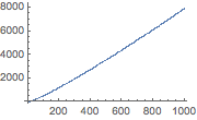
ListPlot is a variant of Plot that just takes a list of values and plots them. For example, let’s plot the first 1000 primes. The function we’re using here, Table , is explained more in the next section.

ListPlot[Table[Prime[n], {n, 1000}],
 ImageSize -> Small]

(*Out:*)

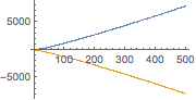
Similarly to Plot , we can plot multiple data sets:

ListPlot[{
  Table[Prime[n], {n, Range[2, 1000, 2]}],
  Table[-Prime[n], {n, Range[1, 999, 2]}]},
 ImageSize -> Small]

(*Out:*)

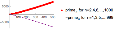
And again we can apply styling rules:

ListPlot[{
  Table[Prime[n], {n, Range[2, 1000, 2]}],
  Table[-Prime[n], {n, Range[1, 999, 2]}]},
 PlotLegends -> {"primen for \
n=2,4,6,...,1000",
   "-primen for n=1,3,5,...,999"},
 PlotStyle -> {Directive[AbsolutePointSize[5], Red], 
   Directive[AbsolutePointSize[.1], Purple]},
 ImageSize -> Small
 ]

(*Out:*)

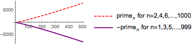
We can also join the points to plot out a line

ListPlot[{
  Table[Prime[n], {n, Range[2, 1000, 2]}],
  Table[-Prime[n], {n, Range[1, 999, 2]}]},
 PlotLegends -> {"primen for \
n=2,4,6,...,1000",
   "-primen for n=1,3,5,...,999"},
 PlotStyle -> {Directive[Dashed, Red], Directive[Thick, Purple]},
 Joined -> True,
 ImageSize -> Small
 ]

(*Out:*)

Plot3D

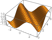
Plot3D works just like Plot , but takes two ranges

Plot3D[Sin[x + y], {x, -π, π}, {y, 0, 2 π},
 ImageSize -> Small]

(*Out:*)

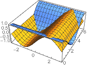
Multiple functions:

Plot3D[{Sin[x], Cos[y]}, {x, -π, π}, {y, 0, 2 π},
 ImageSize -> Small]

(*Out:*)

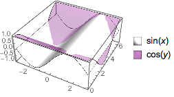
Styling:

Plot3D[{Sin[x], Cos[y]}, {x, -π, π}, {y, 0, 2 π},
 PlotLegends -> "Expressions",
 MeshStyle -> None,
 PlotStyle -> {
   Directive[Specularity[Gray, 10], White],
   Directive[Purple, Specularity[Gray, 100], Opacity[.3]]},
 Lighting -> "Neutral",
 ImageSize -> Small]

(*Out:*)

Special Plots

Mathematica, being the massive system it is, has more-or-less every plot type one could desire built in. Most of these will not be generally useful, but it is worth keeping in mind that any plot type one could want, like, say, a 3D point-wise density-estimating plot, Mathematica has it. See: ListDensityPlot3D .

That specific plot will be useful later in finding local sinks from gradient functions and is not the kind of run-of-the-mill plot one sees everywhere.