‌

Symbolic Algebra

As is explained more fully in the Mathematica Programming section, the language Mathematica is built around is almost 100% symbolic, which makes it perfect for algebraic manipulations.

One of the simplest examples of things one can do in Mathematica is generate and combine polynomials:

simplePolynomial[var_,order_]:=
 Total@Table[RandomInteger[10]*Power[var,n],{n,order}];

pX1=simplePolynomial[x,2]

4 x+6 x2

pX2=simplePolynomial[x,2]

10 x+10 x2

pX1+pX2

14 x+16 x2

This works just as well at any polynomial order. Here we’ll add five randomly generated polynomials of order less than or equal to 15 .

Array[(simplePolynomial[x,RandomInteger[15]])&,5]//Total

22 x+26 x2+15 x3+28 x4+10 x5+9 x6+12 x7+13 x8+19 x9+11 x10+9 x11+13 x12+6 x13+4 x14

For those interested, the & specifies that what comes before should be treated as a function, but absent any variables we simply get our expression as a result.

Simplify

For more complex things we’ll need to explicitly simplify them:

sphericalHarmonicSum=Total@Array[SphericalHarmonicY[RandomInteger[5],RandomInteger[5],θ,ϕ]&,5]

-  ϕ  Sin[θ]+ 2  ϕ  Cos[θ] Sin[θ]2+ 2  ϕ  Cos[θ] (-1+3 Cos[θ]2) Sin[θ]2

We can then have Mathematica simplify this expression for us more:

Simplify[sphericalHarmonicSum]

 ϕ  Sin[θ] (-32+2  (4+)  ϕ Sin[2 θ]+3   ϕ Sin[4 θ])

Sometimes we also need to use the function FullSimplify to get everything simplified:

FullSimplify[sphericalHarmonicSum]

 ϕ  Sin[θ] (-16+  ϕ (4++3  Cos[2 θ]) Sin[2 θ])

It often makes sense to go for Simplify over FullSimplify , despite the fact that we can get more simplification out of FullSimplify , because sometimes the Simplify is all we need to see a pattern ourselves, while FullSimplify can over-simplify and obliterate that pattern.

It’s good to keep in mind that while Mathematica may know more than we do, we're still smarter than it is.

Solve

Mathematica can also solve equations for us. We’ll try this on a nice quartic polynomial:

polynomialInX=simplePolynomial[x, 4]

6 x+5 x2+3 x3+6 x4

Note that there’s no nice way to find the roots of this polynomial by hand. But Mathematica doesn’t mind:

Solve[polynomialInX0,x]

{ {x0},{x (-1-+(-94+)1/3)},{x-+- (1- ) (-94+)1/3},{x-+- (1+ ) (-94+)1/3} }

As mentioned before, Mathematica knows more math than any of us. It sees a quartic polynomial and knows that by the fundamental theorem of algebra there are four solutions to this equation, we just might need to find complex solutions.

Usually this isn’t what we want, unfortunately. Happily Mathematica can dumb itself down for us.

Solve[polynomialInX0,x,Reals]

{ {x0},{xRoot[6+5 #1+3 #12+6 #13&,1]} }

Notice that we get this odd Root expression. That’s the way Mathematica represents a perfectly exact root. We can get its numerical one of two ways. Either we make the equation inexact:

Solve[polynomialInX0., x, Reals]

{ {x-0.867733324263096`},{x0} }

Or we numericize after the fact:

N[Solve[polynomialInX0,x,Reals],6]

One useful thing to know with Solve is why the results are returned so oddly. Each list is a different solution, which is more important with multivariate equations, which we’ll get to, but first let’s see a nice way to get out our solutions in a simple list:

x/.N[Solve[polynomialInX0,x,Reals],6]

(*Out:*)

{0,-0.8677333242630958819`6.}

The /. is an alias for ReplaceAll , which is described in more detail later in the Replacement Patterns section. For now let’s just note that any time it sees var on the left hand side it looks for varval on the right hand side and replaces var with that.

Now let’s also see how we can plot these solutions:

Show[Plot[polynomialInX,{x,-2,2}],ListPlot[Table[{x,0},{x,x/.Solve[polynomialInX0.,x,Reals]}]]]

(*Out:*)

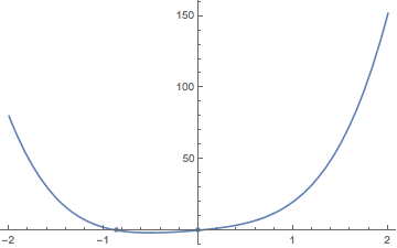
We have to use ListPlot to plot our discrete solutions, but we can see we get the result we expect.

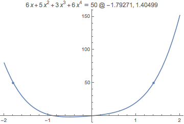
We could even write a function that will solve the equation for an arbitrary value and plot the result:

solveAndPlot[eqInX_,val_]:=Show[Plot[eqInX,{x,-2,2}],ListPlot[Table[{x,val},{x,x/.Solve[eqInX(1.val),x,Reals]}]],PlotLabelRow@{HoldForm[eqInXval]," @ ",Row@Riffle[(x/.Solve[eqInX(1.val),x,Reals]),", "]}];

solveAndPlot[polynomialInX,50]

(*Out:*)

But that’s getting distracted, I suppose.

Multivariate Solve

Let’s move to multivariate equations now:

polynomialInXandY=simplePolynomial[x,3]+simplePolynomial[y,3]

8 x+2 x2+2 y+10 y2+8 y3

It can still solve this equation, although as it will admit, it may miss some solutions.

Solve[polynomialInXandY == 0,{x,y}, Reals]

{ {xConditionalExpression[-2-,y< (-5+(829-6 )1/3+(829+6 )1/3)]},{xConditionalExpression[-2+,y< (-5+(829-6 )1/3+(829+6 )1/3)]},{x-2-√(4+ (5-(829-6 )1/3-(829+6 )1/3)- (-5+(829-6 )1/3+(829+6 )1/3)2- (-5+(829-6 )1/3+(829+6 )1/3)3),y (-5+(829-6 )1/3+(829+6 )1/3)} }

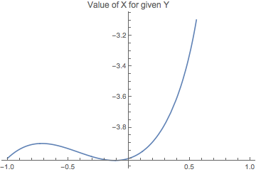
Note that it also gives us these odd ConditionalExpression statements. This is because the solution could branch depending on how x and y interplay. Let’s just get take one of these solutions and plot it:

conditionalSoln=First[x/.Solve[polynomialInXandY == 0.,{x,y}, Reals]];
N[conditionalSoln]

(*Out:*)

ConditionalExpression[-2.`-1.` ,y<0.6609358769285026`]

Plot[conditionalSoln,{y,-1,1},PlotLabel"Value of X for given Y"]

(*Out:*)

We can force a given branch of this conditional expression, however, by telling Mathematica what it can assume.

Assumptions

When Mathematica simplifies an expression it checks what we’ve told it to about the expression. It does that by looking at the value of the variable $Assumptions

$Assumptions

(*Out:*)

True

This is the default value. But we can make it assume things for us. Let’s assume that y satifies our ConditionalExpression

$Assumptions=y<.5

(*Out:*)

y<0.5`

xAndyRoots={x,y}/.Solve[polynomialInXandY == 0,{x,y}, Reals]//First//Simplify

(*Out:*)

{-2-,y}

And when we’re done we simply reset the $Assumptions variable. We can also apply $Assumptions to a single Simplify expression or similar, but I will leave that to you to look up on.